Tensor Flo Ridas: A Journey in ML
Intro to Boosted Trees
What are boosted trees?
The third model we chose to build was a boosted tree model. Similar to random forest, the boosted tree model builds decision trees over a number of iterations. While the random forest utilizes bootstrap resampling (i.e. bagging) and aggregates the predictions across samples, boosted trees learn sequentially. On each iteration, a tree is built to predict the residuals from the tree before, resulting in a slow learning process.
Boosted trees can lead to overfitting of the data if not tuned properly and can be computationally inefficient. A benefit to the boosted tree model, however, is that the model can be stopped when learning does not surpass a specified threshold, preventing it from overfitting. In fact, boosted trees are known for having some of the best out-of-box performance when predicting tabular data. For this reason, we will give it a try.
Data
Import data
Only 1% of the training data was used so the model tuning wasn’t too computationally demanding. The subset data was split into a training set and a testing set. The training set was used to tune the cross-validated models, while the testing set was used to evaluate it’s performance.
# Import joined data file
data <- import(here("data","data.csv"),
               setclass = "tbl_df")

# Subset data
data_sub <- data %>%
  sample_frac(.1)

# Split data
splits <- initial_split(data_sub, strata = "score")
train <- training(splits)
test <- testing(splits)
Specify recipe
Note the recipe is based off the entire set of training data, but only applied to the subset. This is so imputations are not specific to just a sample of the training data.
rec <- recipe(score ~ ., train) %>%
    step_mutate(tst_dt = lubridate::mdy_hm(tst_dt)) %>%
    update_role(contains("id"), ncessch, sch_name, new_role = "id vars") %>%
    step_novel(all_nominal()) %>%
    step_unknown(all_nominal()) %>%
    step_zv(all_predictors()) %>%
    step_normalize(all_numeric(), -all_outcomes(), -has_role("id vars")) %>%
    step_BoxCox(all_numeric(), -all_outcomes(), -has_role("id vars")) %>%
    step_medianimpute(all_numeric(), -all_outcomes(), -has_role("id vars")) %>%
    step_dummy(all_nominal(), -has_role("id vars"), one_hot = TRUE) %>%
    step_zv(all_predictors())
Preprocess data
For the boosted tree model, the xgboost package was used. Since tidymodels was not used, the data had to be preprocessed before fitting the model. Additional steps were also required, including transforming the preprocessed data into a “feature matrix.” This matrix is the input for the model, which only includes predictors. The scores associated with each row were saved separately into a vector called outcome.
Note: Converting data_sub_baked to a matrix converted everything to a character. This was likely because of the tst_dt variable. To transform the data into an acceptable format for the feature matrix, the tst_dt variable was first converted to a numeric type.
# Preprocess data
train_baked <- rec %>%
  prep() %>%
  bake(train)

# Transform tst_dt to numeric
train_baked$tst_dt <- as.numeric(train_baked$tst_dt)

# Transform preprocessed data into feature matrix
features <- train_baked %>%
  select(-score, -contains("id"), -ncessch, -sch_name) %>%
  as.matrix()

# Saving the scores as a separate vector
outcome <- train_baked$score
Model Tuning
Boosted trees have considerably more hyperparameters than random forest. For the purpose of our project, we chose what we felt were the most important hyperparameters:
Number of trees - If too many trees are used, then our model can overfit the data. This would result in poor out-of-box performance. Alternatively, too few trees may not allow our model enough time to learn.
Learning rate - Boosted trees often utilize a learning process called gradient descent. On each iteration, the model is adjusted in a way that most reduces the cost function (e.g. RMSE). The amount in which the model is adjusted on each iteration is determined by the learning rate. When the learning rate is high, the model can make adjustments that are too large and end up being far from the optimal solution. When the learning rate is too low, the model may not reach the optimal solution within the specified number of trees.
Tree depth - This refers to the number of splits for each tree. In contrast to random forest, shallow trees are used, typically with 1 to 6 splits. A shallower tree would require more trees to reach the optimal solution, while a deeper tree can lead to overfitting.
Randomness - There are a number of ways in which randomness can be introduced to a boosted tree model. One is sampling the number of predictors used to determine each split within a tree. This is similar to the random forest model, in which the number of predictors sampled for each tree (
mtry) is a hyperparameter.
Basic model without any tuning
Before tuning the boosted tree model, a single-cross validated model with default hyperparameters was run to estimate the timing.
The default boosted * 100 trees * early stop after 20 iterations of no learning * 10-fold cross validation
tic()

fit_def_xgb <- xgb.cv(
  data = features,
  label = outcome,
  nrounds = 100,
  objective = "reg:squarederror",
  early_stopping_rounds = 20,
  nfold = 10,
  verbose = 0
)

time_default <- toc()
## 32.344 sec elapsedNote the cross-validated boosted tree model with default parameters took about 42.467 s. Will proceed with caution.
Below are the mean train and test metrics from each iteration (i.e. tree). The model is evaluated using root mean squared error (RMSE).
fit_def_xgb$evaluation_logfit_def_log <- fit_def_xgb$evaluation_log %>%
pivot_longer(-iter,
names_to = c("set","metric","measure"),
names_sep = "_") %>%
pivot_wider(names_from = "measure",
values_from = "value") %>%
filter(iter > 5)
ggplot(fit_def_log, aes(iter, mean)) +
geom_line(aes(color = set), size = 1) +
labs(x = "Tree Iteration", y = "Mean RMSE") +
scale_color_manual(values = c("#FFDB6D", "#00AFBB")) +
theme_407()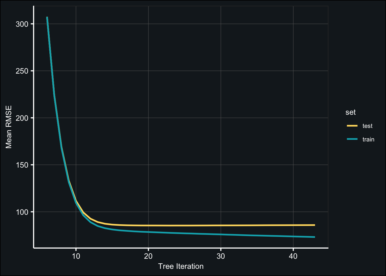
fit_def_xgb$best_iteration## [1] 23fit_def_xgb$evaluation_log %>%
dplyr::slice(fit_def_xgb$best_iteration)mt_rmse <- fit_def_xgb$evaluation_log %>%
dplyr::slice(fit_def_xgb$best_iteration) %>%
select(test_rmse_mean)Even with the default parameters, the mean RMSE across the test sets is relatively good (85.34). Let’s see how well the model will do with some tuning!
Tune number of trees
- start at high learning rate (shrinkage = .1)
grid_tree = expand.grid(num_tree = seq(100, 1000, length.out = 5))

tic()
fit_tune_trees <- map(grid_tree$num_tree, ~ {
 xgb.cv(
   data = features,
   label = outcome,
   nrounds = .x, # number of trees
   objective = "reg:squarederror",
   early_stopping_rounds = 20,
   nfold = 10,
   params = list(eta = .1),
   verbose = 0
 )
})
toc()
## 350.766 sec elapsedBelow are the results of the tuned models:
fit_tune_tree_log <- map_df(fit_tune_trees, ~{
  .x$evaluation_log %>%
  pivot_longer(-iter,
               names_to = c("set","metric","measure"),
               names_sep = "_") %>%
  pivot_wider(names_from = "measure",
              values_from = "value")
}, .id = "num_tree") %>%
  mutate(num_tree = factor(num_tree,
                           labels = str_c(as.character(grid_tree$num_tree), "trees", sep = " "))) %>%
  filter(iter > 30)

ggplot(fit_tune_tree_log, aes(iter, mean)) +
  geom_line(aes(color = set), size = 1) +
  labs(x = "Tree Iteration", y = "Mean RMSE") +
  scale_color_manual(values = c("#FFDB6D", "#00AFBB")) +
  theme_407() +
  facet_grid(~num_tree) +
  theme(axis.text.x = element_text(size = 8))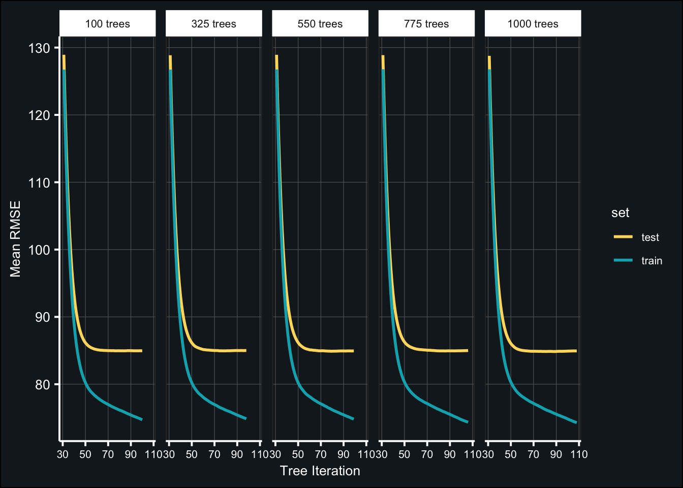
(tune_tree_best <- map_df(fit_tune_trees, ~{
  .x$evaluation_log %>%
  dplyr::slice(.x$best_iteration)
}) %>%
  mutate(num_trees = grid_tree$num_tree) %>%
  arrange(test_rmse_mean) %>%
  select(num_trees, iter, test_rmse_mean, test_rmse_std))
best_numtrees <- tune_tree_best$num_trees[1]Tune learning rate (pt. 1)
Typical learning rate is .001 - .3
- use optimal number of trees
grid_learn <- expand.grid(learn_rate = seq(.001, .3, length.out = 10))

tic()
fit_tune_learn1 <- map(grid_learn$learn_rate, ~ {
 xgb.cv(
   data = features,
   label = outcome,
   nrounds = 100, # number of trees
   objective = "reg:squarederror",
   early_stopping_rounds = 20,
   nfold = 10,
   params = list(eta = .x),
   verbose = 0
 )
})
toc()
## 516.128 sec elapsedBelow are the results of the tuned models:
fit_tune_learn1_log <- map_df(fit_tune_learn1, ~{
  .x$evaluation_log %>%
  pivot_longer(-iter,
               names_to = c("set","metric","measure"),
               names_sep = "_") %>%
  pivot_wider(names_from = "measure",
              values_from = "value")
}, .id = "learn_rate") %>%
  mutate(learn_rate = factor(learn_rate,
                             levels = as.character(seq(1,10)),
                             labels = as.character(round(grid_learn$learn_rate,3)))) %>%
  filter(iter > 10)

ggplot(fit_tune_learn1_log, aes(iter, mean)) +
  geom_line(aes(color = set), size = 1) +
  labs(x = "Tree Iteration", y = "Mean RMSE") +
  scale_color_manual(values = c("#FFDB6D", "#00AFBB")) +
  theme_407() +
  facet_wrap(~learn_rate, nrow = 2) +
  theme(axis.text.x = element_text(size = 6))
(tune_learn1_best <- map_df(fit_tune_learn1, ~{
  .x$evaluation_log %>%
  dplyr::slice(.x$best_iteration)
}) %>%
  mutate(learning_rate = grid_learn$learn_rate) %>%
  arrange(test_rmse_mean) %>%
  select(learning_rate, iter, test_rmse_mean, test_rmse_std))
best_learnrate1 <- tune_learn1_best$learning_rate[1]Tune tree depth
- use optimal number of trees
- use optimal learning rate
Defined as max_depth in XGBoost
grid_depth <- expand.grid(tree_depth = seq(1,6))

tic()
fit_tune_depth <- map(grid_depth$tree_depth, ~ {
 xgb.cv(
   data = features,
   label = outcome,
   nrounds = best_numtrees, # number of trees
   objective = "reg:squarederror",
   early_stopping_rounds = 20,
   nfold = 10,
   params = list(eta = best_learnrate1,
                 max_depth = .x),
   verbose = 0
 )
})
toc()
## 629.672 sec elapsedBelow are the results of the tuned models:
fit_tune_depth_log <- map_df(fit_tune_depth, ~{
  .x$evaluation_log %>%
  pivot_longer(-iter,
               names_to = c("set","metric","measure"),
               names_sep = "_") %>%
  pivot_wider(names_from = "measure",
              values_from = "value")
}, .id = "tree_depth") %>%
  filter(iter > 20)

ggplot(fit_tune_depth_log, aes(iter, mean)) +
  geom_line(aes(color = set), size = 1) +
  labs(x = "Tree Iteration", y = "Mean RMSE") +
  scale_color_manual(values = c("#FFDB6D", "#00AFBB")) +
  theme_407() +
  facet_grid(~tree_depth) +
  theme(axis.text.x = element_text(size = 6))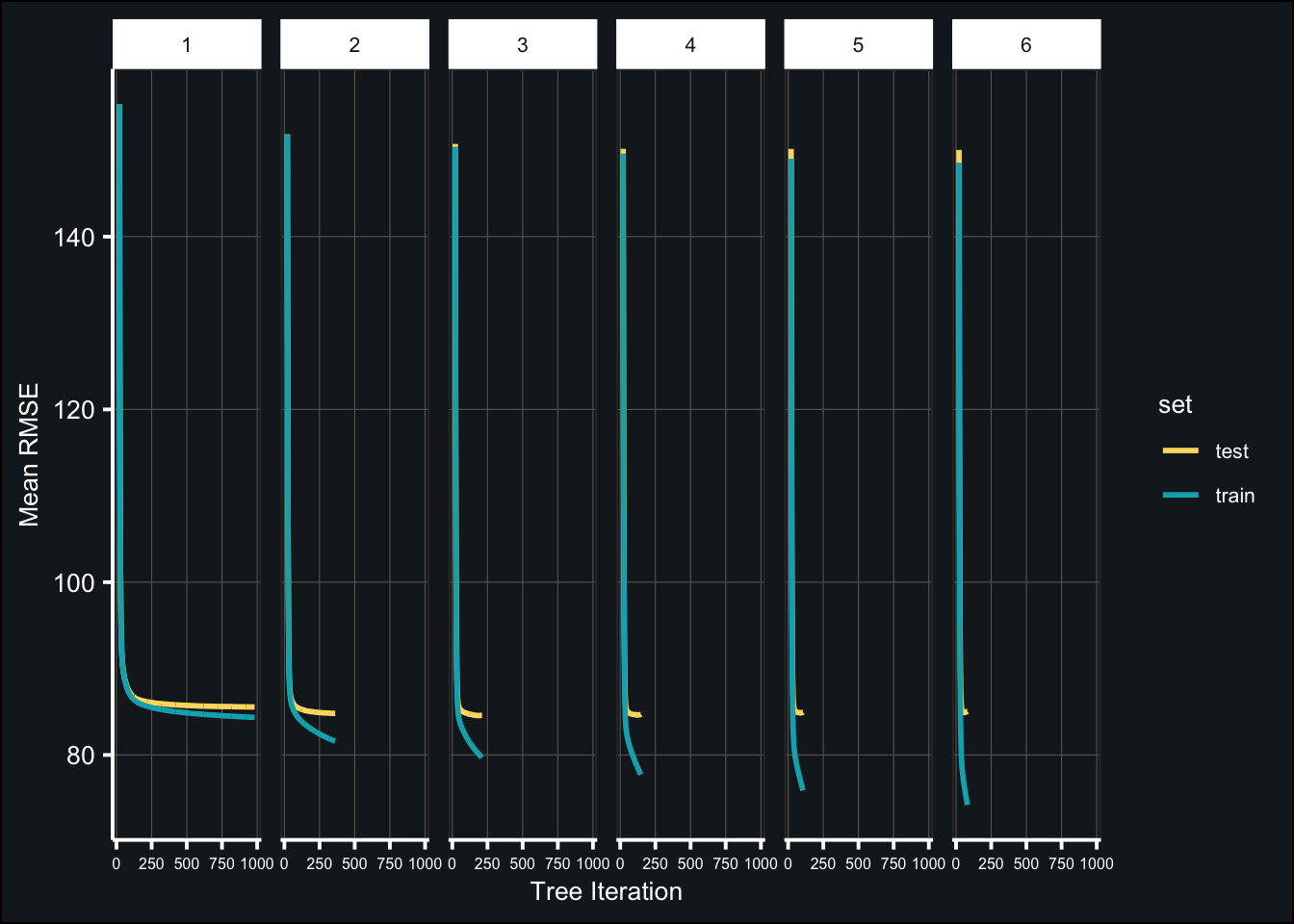
(tune_depth_best <- map_df(fit_tune_depth, ~{
  .x$evaluation_log %>%
  dplyr::slice(.x$best_iteration)
}) %>%
  mutate(tree_depth = grid_depth$tree_depth) %>%
  arrange(test_rmse_mean) %>%
  select(tree_depth, iter, test_rmse_mean, test_rmse_std))
best_depth<- tune_depth_best$tree_depth[1]Tune randomness
- use optimal number of trees
- use optimal learning rate
- use optimal tree depth
Defined as colsample_bytree in XGBoost This parameter determines the number of features to sample for each new tree, similar to mtry in tidymodels.
grid_randcol <- expand.grid(colsample = seq(.1, 1, length.out = 5))

tic()
fit_tune_randcol <- map(grid_randcol$colsample, ~ {
 xgb.cv(
   data = features,
   label = outcome,
   nrounds = best_numtrees, # number of trees
   objective = "reg:squarederror",
   early_stopping_rounds = 20,
   nfold = 10,
   params = list(eta = best_learnrate1,
                 max_depth = best_depth,
                 colsample_bytree = .x),
   verbose = 0
 )
})
toc()
## 358.136 sec elapsedBelow are the results of the tuned models:
fit_tune_randcol_log <- map_df(fit_tune_randcol, ~{
  .x$evaluation_log %>%
  pivot_longer(-iter,
               names_to = c("set","metric","measure"),
               names_sep = "_") %>%
  pivot_wider(names_from = "measure",
              values_from = "value")
}, .id = "col_sample") %>%
  mutate(col_sample = factor(col_sample,
                             labels = as.character(grid_randcol$colsample))) %>%
  filter(iter > 25)

ggplot(fit_tune_randcol_log, aes(iter, mean)) +
  geom_line(aes(color = set), size = 1) +
  labs(x = "Tree Iteration", y = "Mean RMSE") +
  scale_color_manual(values = c("#FFDB6D", "#00AFBB")) +
  theme_407() +
  facet_grid(~col_sample) +
  theme(axis.text.x = element_text(size = 6))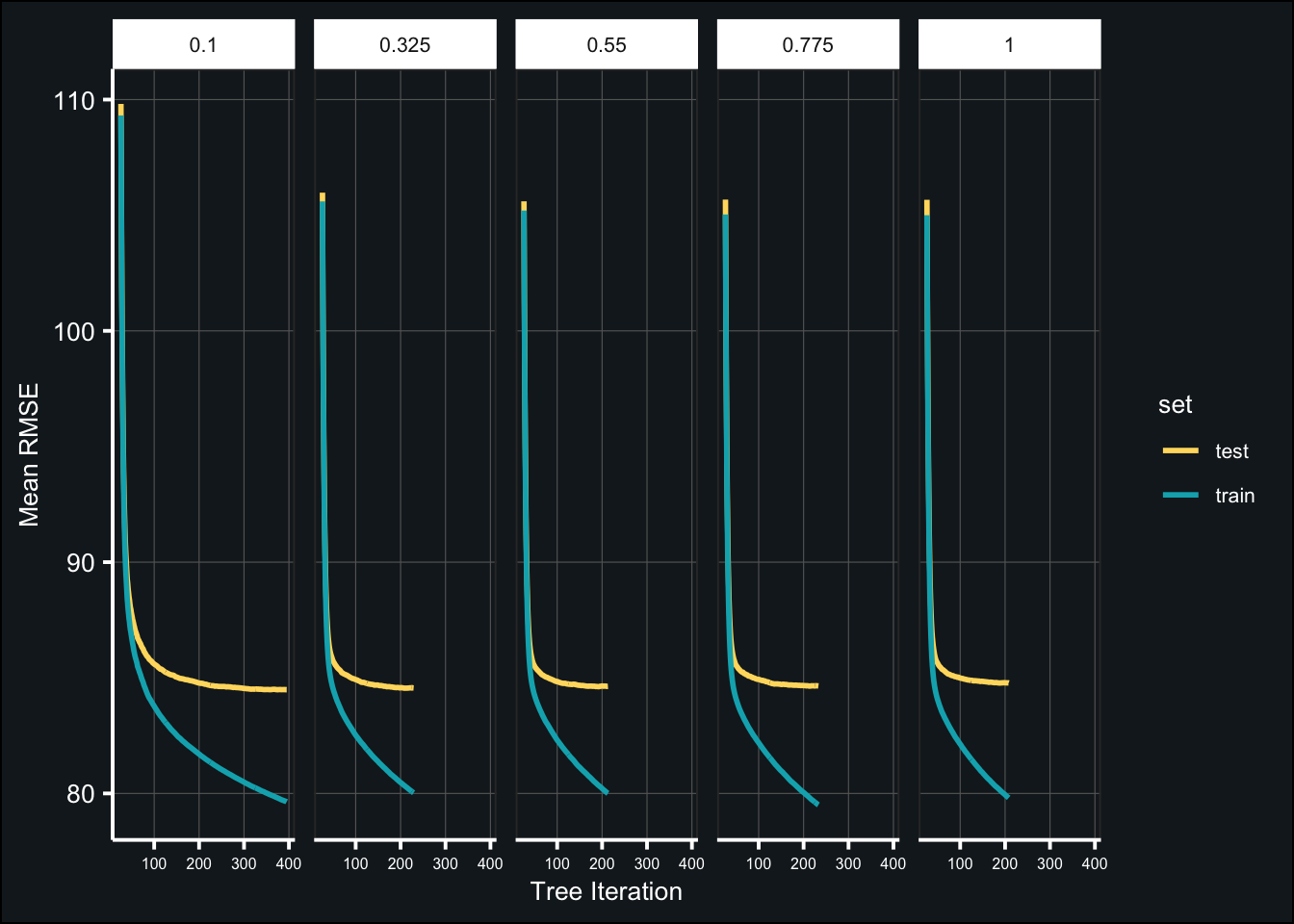
(tune_randcol_best <- map_df(fit_tune_randcol, ~{
  .x$evaluation_log %>%
  dplyr::slice(.x$best_iteration)
}) %>%
  mutate(colsample = grid_randcol$colsample) %>%
  arrange(test_rmse_mean) %>%
  select(colsample, iter, test_rmse_mean, test_rmse_std))
best_colsample <- tune_randcol_best$colsample[1]Tune learning rate (pt. 2)
- use optimal tree parameters
- use optimal number of trees
- tune using lower learning rates
grid_learn <- expand.grid(learn_rate = seq(.001, .15, length.out = 5))

tic()
fit_tune_learn2 <- map(grid_learn$learn_rate, ~ {
 xgb.cv(
   data = features,
   label = outcome,
   nrounds = best_numtrees, # number of trees
   objective = "reg:squarederror",
   early_stopping_rounds = 20,
   nfold = 10,
   params = list(eta = .x,
                 max_depth = best_depth,
                 colsample_bytree = best_colsample),
   verbose = 0
 )
})
toc()
## 577.299 sec elapsedBelow are the results of the tuned models:
fit_tune_learn2_log <- map_df(fit_tune_learn2, ~{
  .x$evaluation_log %>%
  pivot_longer(-iter,
               names_to = c("set","metric","measure"),
               names_sep = "_") %>%
  pivot_wider(names_from = "measure",
              values_from = "value")
}, .id = "learn_rate") %>%
  mutate(learn_rate = factor(learn_rate,
                             labels = as.character(round(grid_learn$learn_rate,3)))) %>%
  filter(iter > 10)

ggplot(fit_tune_learn2_log, aes(iter, mean)) +
  geom_line(aes(color = set), size = 1) +
  labs(x = "Tree Iteration", y = "Mean RMSE") +
  scale_color_manual(values = c("#FFDB6D", "#00AFBB")) +
  theme_407() +
  facet_grid(~learn_rate) +
  theme(axis.text.x = element_text(size = 8))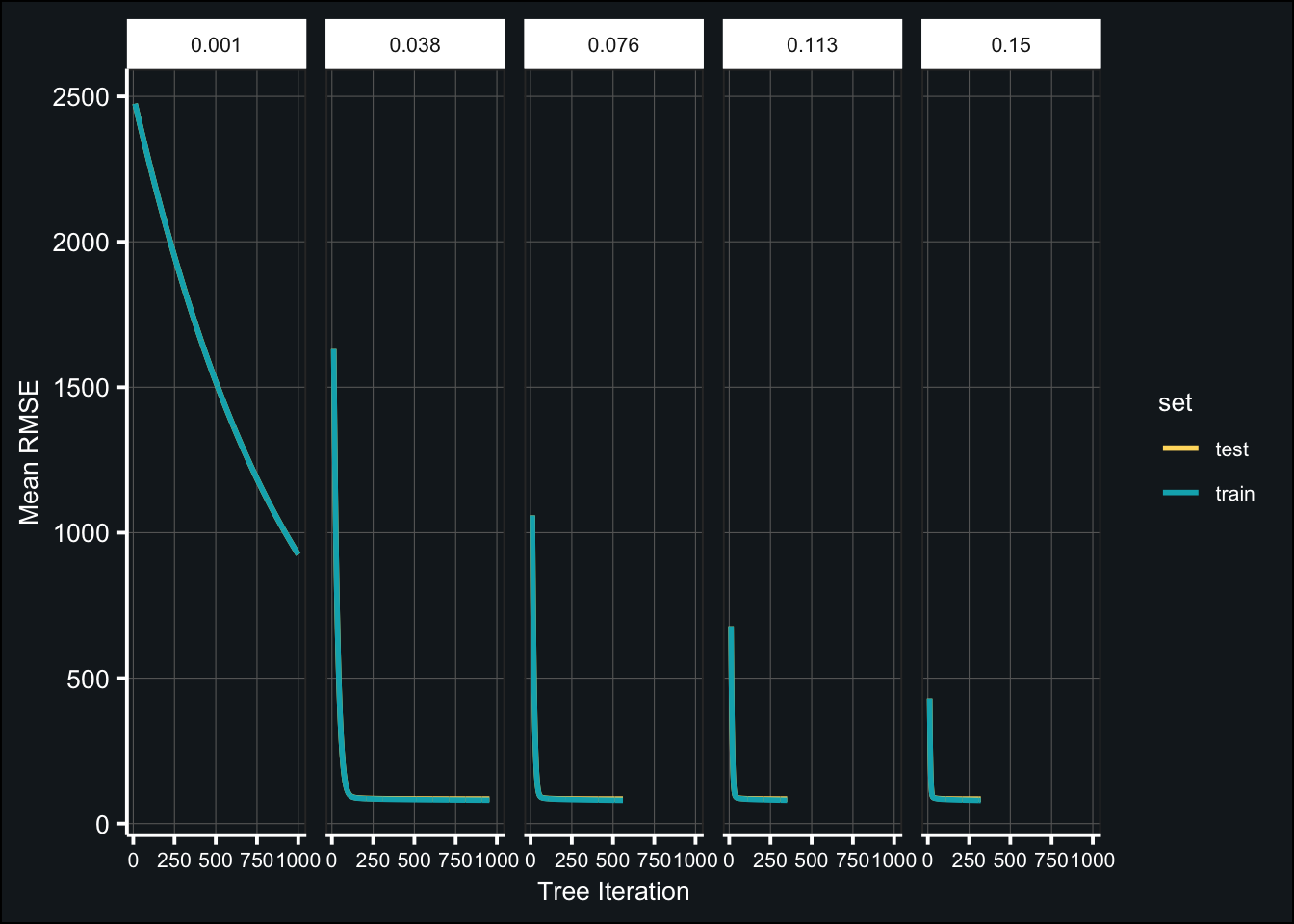
(tune_learn2_best <- map_df(fit_tune_learn2, ~{
  .x$evaluation_log %>%
  dplyr::slice(.x$best_iteration)
}) %>%
  mutate(learning_rate = grid_learn$learn_rate) %>%
  arrange(test_rmse_mean) %>%
  select(learning_rate, iter, test_rmse_mean, test_rmse_std))
best_learnrate2 <- tune_learn2_best$learning_rate[1]Fit the final model
Finalize model
The final model using the optimal hyperparameters was trained on the training set.
tic()

fit_final_xgb <- xgboost(
   data = features,
   label = outcome,
   nrounds = best_numtrees, # number of trees
   objective = "reg:squarederror",
   early_stopping_rounds = 20,
   params = list(eta = best_learnrate2,
                 max_depth = best_depth,
                 colsample_bytree = best_colsample),
   verbose = 0
 )

toc()
## 19.097 sec elapsedPreprocess test split
The testing set was preprocessed using the same recipe as the training data.
# Preprocess data
test_baked <- rec %>%
  prep() %>%
  bake(test)

# Transform tst_dt to numeric
test_baked$tst_dt <- as.numeric(test_baked$tst_dt)

# Transform preprocessed data into feature matrix
test_data <- test_baked %>%
  select(-score, -contains("id"), -ncessch, -sch_name) %>%
  as.matrix()

# Saving the scores as a separate vector
test_outcome <- test_baked$score
Test final model
The final model was used to make predictions in the testing set. The performance of the model was evaluated using RMSE.
# Make predictions
predictions <- predict(fit_final_xgb, test_data)

# Calculate RMSE
pred_tbl <- tibble(predictions, test_outcome)
(test_rmse <- yardstick::rmse(pred_tbl, predictions, test_outcome))
Final thoughts
The final RMSE on the assessment set was relatively good at 85.76. However, this isn’t far off from the mean RMSE when cross-validating a boosted tree model using the default parameters, 85.34. This finding suggests tuning did not add any predictive power to our model. Given that each tuning step took about 3 - 10 minutes, the change in RMSE does not seem worth the additional effort. There are a number of other hyperparameters that can be tuned in boosted tree models, including minimum n for each node in a tree or thresholding the change in cost function before stopping a tree. It is possible these additional parameters would have improved the performance of our model. Overall, though the boosted tree model demonstrated low variance and had relatively good predictive power, it was computationally inefficient in terms of how many hyperparameters can be tuned and how long it takes to tune, even with just 10% of the data.