Tensor Flo Ridas: A Journey in ML
The outcome variable
Across the entire United States, students in grades 3-8 are tested annually in reading and math. Our goal in this course was to create a machine learning model capable of accurately predicting a given student’s performance on these tests (i.e., a scaled test total score). While our dataset is simulated from actual statewide testing administration across the state of Oregon, the overall distributions are highly similar. The school IDs (ncessch) are real. So we used school IDs to link our simulated data with other sources (e.g., National Center for Educational Statistics), which will be elaborated upon below.
Simulated data predictors
As mentioned above, our dataset simulates real testing data in the state of Oregon. Below is a summary of the 39 predictor variables included in this dataset:
dictionary <- import(here::here("data", "ASHdata_dictionary.xlsx"),
                     setclass = "tbl_df")
dictionary %>%
  kbl() %>%
  kable_styling(bootstrap_options = c("condensed", "responsive"),
                full_width = F) %>%
  row_spec(0, background = "#171F24", color = "white") %>% # Color header row background
  column_spec(1, bold = T, border_right = T, background = "#171F24", color = "white") %>%
  column_spec(2, width = "40em", background = "#171F24", color = "white") %>%
scroll_box(width = "100%", height = "225px")| Variable Name | Description |
|---|---|
| id | Unique student identifier |
| gndr | Code indicating the gender of the student |
| ethnic_cd | Code representing the racial/ethnic reporting subgroup category for the student |
| attnd_dist_inst_id | The District where the student is receiving instruction and where state assessments are administered |
| attnd_schl_inst_id | The School where the student is receiving instruction and where state assessments are administered |
| enrl_grd | Enrolled grade level of the student |
| calc_admn_cd | Special circumstances affecting test administration (e.g., home schooled, foreign exchange, out of state) |
| tst_bnch | Benchmark level of the administered test (e.g., grade 3, grade 5, grade 8) |
| tst_dt | Date the test was taken (mm/dd/yyyy) |
| migrant_ed_fg | Student participation in a program designed to assure that migratory children receive full and appropriate opportunities |
| ind_ed_fg | Student participation in a program designed to meet educational and culturally related academic needs of American Indians |
| sp_ed_fg | Student participation in an Individualized Education Plan (IEP/IFSP) |
| tag_ed_fg | Student participation in a Talented and Gifted program |
| econ_dsvntg | Student eligibility for a Free or Reduced Lunch program |
| ayp_lep | Student who received services (or was eligible to receive services) in a Limited English Proficient program |
| stay_in_dist | Student enrolled > 50% of the days in the school year at the district where the student is resident |
| stay_in_schl | Student enrolled > 50% of the days in the school year at the school where the student is resident |
| dist_sped | Student enrolled in a district special education program and received general education classroom instruction < 40% of the time |
| trgt_assist_fg | Record is included in Title 1 Targeted Assistance for the Adequate Yearly Progress (AYP) school performance calculations |
| ayp_dist_partic | Record is included in the denominator of Adequate Yearly Progress (AYP) district participation calculations |
| ayp_schl_partic | Record is included in the denominator of Adequate Yearly Progress (AYP) school participation calculations |
| ayp_dist_prfrm | Record is included in the denominator of Adequate Yearly Progress (AYP) district performance calculations |
| ayp_schl_prfrm | Record is included in the denominator of Adequate Yearly Progress (AYP) school performance calculations |
| rc_dist_partic | Record is included in the denominator of Report Card (RC) district participation calculations |
| rc_schl_partic | Record is included in the denominator of Report Card (RC) school participation calculations |
| rc_dist_prfrm | Record is included in the denominator of Report Card (RC) district performance calculations |
| rc_schl_prfrm | Record is included in the denominator of Report Card (RC) school participation calculations |
| partic_dist_inst_id | The Resident District where the student was enrolled on the first school day in May. |
| partic_schl_inst_id | The Resident School where the student was enrolled on the first school day in May. |
| lang_cd | Language of the test (English or Spanish) |
| tst_atmpt_fg | Code describing whether the test was attempted |
| grp_rpt_dist_partic | Record is included in the denominator of Group Report district participation calculations |
| grp_rpt_schl_partic | Record is included in the denominator of Group Report school participation calculations |
| grp_rpt_dist_prfrm | Record is included in the denominator of Group Report district performance calculations |
| grp_rpt_schl_prfrm | Record is included in the denominator of Group Report school participation calculations |
| classification | Performance Level for Benchmark (PLB) Total Score |
| ncessch | NCES school identifier |
| lat | school latitute |
| lon | school longitute |
\(~\)
And below you can find a summary of the descriptive statistics for each variable:
# read in data set
data <- read_csv("data/train.csv",
                 col_types = cols(.default = col_guess(),
                                  calc_admn_cd = col_character())) %>%
    select(-classification)

psych::describe(data)
\(~\)
Additional data sources
Free and reduced lunch
Note that our simulated dataset described above primarily includes student-level predictors. We decided to import additional data containing info specific to the schools (ncessch) students attend. We reasoned that school-level variables could have an important impact on the quality of education students receive, in turn impacting students’ scores.
First, we obtained free/reduced lunch data for each school and counted the number of students at each school. In doing so, our goal was to create two new predictor variables that we could add to our existing dataset. Namely, we computed variables that reflect the proportion of students at a given school who are eligible for free (free_lunch_prop) or reduced (reduced_lunch_prop) lunches.
# read in free/reduced lunch data and student counts
frl <- import(here("data", "lunch.csv"),
              setclass = "tbl_df")  %>%
  janitor::clean_names()  %>%
  filter(st == "OR")  %>%
  select(ncessch, lunch_program, student_count)  %>%
  mutate(student_count = replace_na(student_count, 0))  %>%
  pivot_wider(names_from  = lunch_program,
              values_from = student_count)  %>%
  janitor::clean_names()  %>%
  mutate(ncessch = as.double(ncessch))

stu_counts <- import("https://github.com/datalorax/ach-gap-variability/raw/master/data/achievement-gaps-geocoded.csv",
                     setclass = "tbl_df")  %>%
  filter(state == "OR" & year == 1718)  %>%
  count(ncessch, wt = n)  %>%
  mutate(ncessch = as.double(ncessch))

frl <- left_join(frl, stu_counts)

rm(stu_counts)

frl <- frl %>%
  mutate(free_lunch_prop = free_lunch_qualified / n,
         reduced_lunch_prop = reduced_price_lunch_qualified / n)  %>%
  select(ncessch, ends_with("prop"))

psych::describe(frl)
\(~\)
Staff
Here we obtained data on the number of full-time-equivalent (FTE) teachers at each school (teachers). Schools with more funding seemingly offer more resources and newer, better equipment for students–possibly contributing to better test scores. Our rationale was that the number of full-time teachers at a school could potentially serve as an indirect index of school funding. Or, perhaps the number of full time teachers could be negatively associated with class room size. If smaller class rooms are associated with better student performance, then perhaps this is another means by which the number of full-time teachers could aid in the predictive utility of our model.
# read in staff data
staff <- import(here("data", "staff.csv"), setclass = "tbl_df")  %>%
  janitor::clean_names()  %>%
  filter(st == "OR")  %>%
  mutate(ncessch = as.double(ncessch)) %>%
  select(ncessch, teachers)

psych::describe(staff)
\(~\)
Other school characteristics
Here, we sought to add three more predictors. The first, titlei_status refers to a given school’s Title I status. The premise of Title I is that schools with large numbers of low-income students will receive supplemental funds to help ensure that all children meet challenging state academic standards. Note schools may receive a classification other than being a Title I school or not being a Title I school. Schools may also be classified as Title I school-wide eligible + Title I targeted assistance program schools, Title I school-wide eligible + no program schools, and more.
The second predictor of interest was nslp_status, which reflects a given school’s National School Lunch Program (NSLP) status. The NSLP “is a federally assisted meal program operating in public and nonprofit private schools and residential child care institutions”. Children from families with incomes at or below 130% of the Federal Poverty Level (FPL) are eligible for free school meals, whereas children from families with incomes between 130% to 185% FPL qualify for reduced-price meals. Approximately 95% of public schools participate in NSLP in some way. Schools may fall under codes reflecting participation in NSLP without using any Provision or Community Eligibility Option, participation in NSLP under Community Eligibility Option, participation in NSLP under Provision 1, etc.
The final predictor, virtual, refers to a school’s virtual (online) status. Some schools may be fully virtual, not virtual at all, supplemental virtual, or virtual with face to face options.
# read in school characteristics data
school_chars <- import(here("data", "school_characteristics.csv"),
                       setclass = "tbl_df")  %>%
  janitor::clean_names()  %>%
  filter(st == "OR")  %>%
  mutate(ncessch = as.double(ncessch)) %>%
  select(ncessch, titlei_status, nslp_status, virtual)

psych::describe(school_chars)
\(~\)
Ethinicity
Finally, we imported data that breaks down the ethnicity makeup of the students enrolled at each school. Specifically, for each school, we know the proportion of students who identify as:
- American Indian/Alaska Native (
p_american_indian_alaska_native) - Asian (
p_asian) - African American (
p_black_african_american) - Hispanic/Latino (
p_hispanic_latino) - Native Hawaiian/Pacific Islander (
p_native_hawaiian_pacific_islander) - White (
p_white) - Multiracial (
p_multiracial)
# read in ethnicity data
eth <- import(file = here::here("data",
                                "fallmembershipreport_20192020.xlsx"),
              sheet = "School (19-20)",
              setclass = "tibble") %>%
  janitor::clean_names() %>%
  select(attnd_schl_inst_id = attending_school_id,
         sch_name = school_name,
         matches("percent"))

names(eth) <- gsub("x2019_20_percent", "p", names(eth))

psych::describe(eth)
\(~\)
Now we can merge our datasets into a single file whereby cases are matched by school ID (ncessch).
# combine our data with frl, staff, school characteristics, and ethnicities
data <- data %>%
    left_join(frl) %>%
    left_join(staff) %>%
    left_join(school_chars) %>%
    left_join(eth)

# remove unneeded dataframes
rm(frl, staff, school_chars, eth)

head(data)
\(~\)
Data splitting process
Create initial splits
The goal of machine learning is to predict results based on new (unseen) data. The simplest way to do this is to split our merged data into two parts: a training set and a testing set. By default, initial_split() will randomly assign 75% of the merged data to the training set and 25% of the merged data to the testing set.
Training set: These data are used to train our algorithms, tune hyperparameters, compare models, and all of the other tasks necessary to select a final model (e.g., the model we want to put into production). See here for more details.
Testing set: These data are used to estimate an unbiased assessment of the final model’s performance.
Note that after the initial_split(), we use two more rsample functions to create data frames for our training and testing sets. We will eventually fit a series of models (a linear model, random forest model, and a boosted tree model) to the training set and predict the results of the testing set.
set.seed(3000)
data_split <- initial_split(data)
data_train <- training(data_split)
data_test  <- testing(data_split)
\(~\)
Resample training set
Now we need to resample our training set, data_train, to create subsets of “new” data samples that we can train the models on. The most common method–which we use here–is 10-fold cross-validation. Using vfold_cv(), we randomly split the training data into 10 distinct samples (i.e., folds) of approximately equal size. Importantly, each fold contains a sample in which none of the observations are repeated in other folds. And, within each fold, a random 10% of data are sampled for the assessment/testing set (i.e., used to validate model performance), whereas the remaining 90% of the data serve as the analysis/training set in the fold.
set.seed(3000)
data_train_cv <- vfold_cv(data_train)
\(~\)
Feature engineering
Data exploration
First, we wanted to examine the zero order correlations among all continuous variables in the training data. This was done merely for curiosity sake–we were interested in observing which of the 13 continuous predictors were most strongly associated with our outcome variable, score.
- Note: Our dataset has 53 total variables, 1 of which is the outcome variable, and 13 of which are continuous predictors. This means the remaining 39 variables are categorical predictors (7 of which are ID variables).
cor_data <- data_train %>%
  select(where(is.numeric),
         -contains("id"),
         -ncessch) %>%
  cor(use = "pairwise.complete.obs") %>%
  data.frame() %>%
  rownames_to_column() %>%
  gather("colname", "cor", -rowname)

ggplot(cor_data, aes(x = rowname, y = colname, fill = cor)) +
    geom_tile(color = "white") +
    geom_text(aes(label=round(cor,2))) +
    scale_fill_gradient2(low = "#FCCF47",
                         mid = "white",
                         high = "#01C0C0") +
    theme_tensor_flo() +
    theme(axis.text.x = element_text(angle = 45, hjust = 1),
          axis.text = element_text(size = 10.5)) +
    labs(y = "Variable",
         x = "Variable")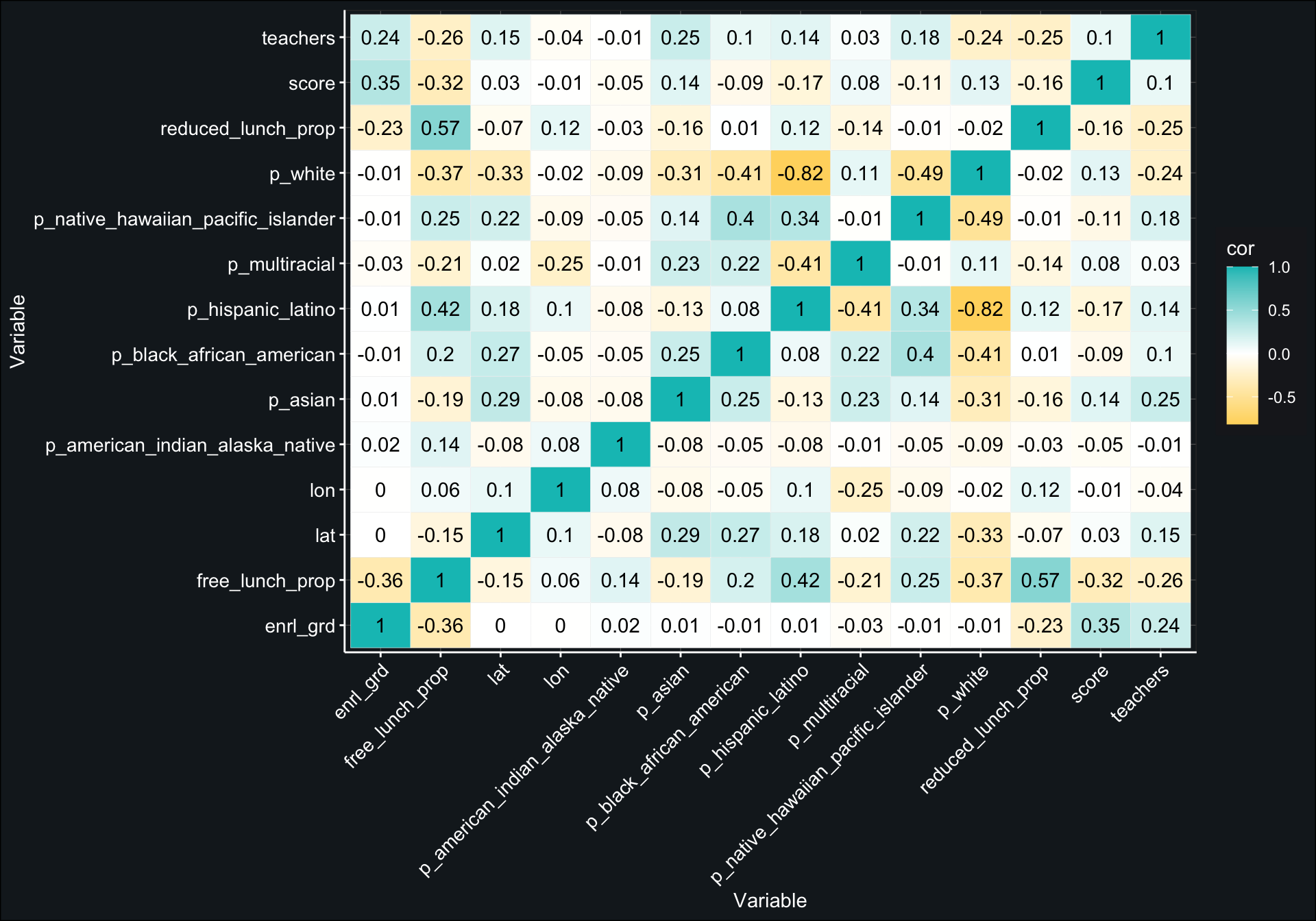
It looks like the two variables most strongly associated with student test performance are the student’s enrolled grade level (enrl_grd) and the proportion of students who qualify for free lunch at the student’s school (free_lunch_prop). Test scores tend to increase as grade level increases, and test scores tend to decline if their school has a larger proportion of students who qualify for free lunch.
Now let’s begin preparing our data for analysis. While we generated descriptive statistics for all variables of interest above, it could be more helpful to examine an array of histograms for our continuous variables. In doing so, we can get a better idea of (1) the range of values for each variable and (2) whether we need to correct for non-normal distributions.
hist_data <- data_train %>%
  select(where(is.numeric),
         -contains("id"),
         -ncessch) %>%
  dplyr::rename("Grade" = `enrl_grd`,
                "Latitude" = `lat`,
                "Longitude" = `lon`,
                "Score" = `score`,
                "Number of Teachers" = `teachers`,
                "Proportion Free Lunch" = `free_lunch_prop`,
                "Proportion Reduced Lunch" = `reduced_lunch_prop`,
                "Proportion Indigenous" = `p_american_indian_alaska_native`,
                "Proportion Asian" = `p_asian`,
                "Proportion African American" = `p_black_african_american`,
                "Proportion Hispanic" = `p_hispanic_latino`,
                "Proportion Pacific Islander" = `p_native_hawaiian_pacific_islander`,
                "Proportion Multiracial" = `p_multiracial`,
                "Proportion White" = `p_white`) %>%
  gather("variable")

ggplot(hist_data, aes(x = value)) +
    geom_histogram(color = "#171f24",
                   fill = "cyan3",
                   alpha = 0.70) +
    facet_wrap(~variable,
               ncol = 4,
               scales = "free") +
    theme_bw() +
    theme_tensor_flo() +
    labs(y = "Count",
         x = "Value")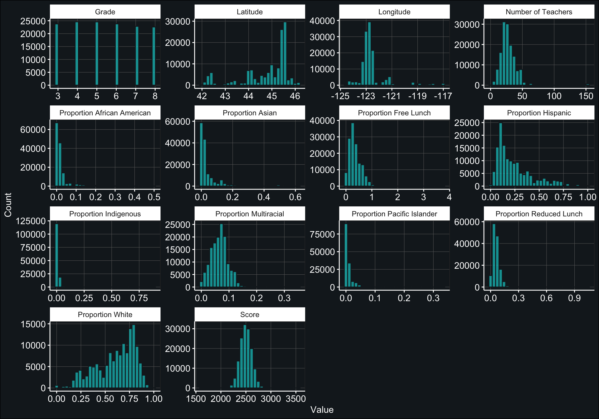
Our outcome variable, score, appears to be normally distributed, but it looks like some of our continuous predictor variables are heavily skewed (e.g., Proportion African American, Proportion Asian, Latitude, etc.) and will definitely need to be transformed. We can address this in our recipe below.
\(~\)
Build the preliminary recipe
Recipes help us preprocess the data by allowing us to make modifications to our data before conducting any formal analysis. Basically, recipes serve as a blueprint outlining any operations we want to apply to a given dataset without actually applying any operations. We then iteratively apply this “blueprint” across sets of data (e.g., folds) during training as well as on new, unseen testing data that has the same variables. This process helps avoid data leakage.
Considering missing data are present, we specified a recipe that used median imputation for missing numerical data. For missing nominal/categorical data, we added an unknown factor level (i.e., role) for said data. Non-normal distributions will be transformed with a box cox transformation. See below where we prep() our recipe for a description of all features of our recipe.
recipe_1 <- recipe(score ~ ., data_train) %>%
    step_mutate(tst_dt = lubridate::mdy_hm(tst_dt)) %>%
    update_role(contains("id"), ncessch, sch_name, new_role = "id vars") %>%
    step_novel(all_nominal()) %>%
    step_unknown(all_nominal()) %>%
    step_zv(all_predictors()) %>%
    step_normalize(all_numeric(), -all_outcomes(), -has_role("id vars")) %>%
    step_BoxCox(all_numeric(), -all_outcomes(), -has_role("id vars")) %>%
    step_medianimpute(all_numeric(), -all_outcomes(), -has_role("id vars")) %>%
    step_dummy(all_nominal(), -has_role("id vars"), one_hot = TRUE) %>%
    step_zv(all_predictors())

prepped_rec <- prep(recipe_1)

prepped_rec
## Data Recipe
##
## Inputs:
##
## role #variables
## id vars 7
## outcome 1
## predictor 45
##
## Training data contained 142176 data points and 142176 incomplete rows.
##
## Operations:
##
## Variable mutation for tst_dt [trained]
## Novel factor level assignment for gndr, ethnic_cd, calc_admn_cd, ... [trained]
## Unknown factor level assignment for gndr, ethnic_cd, calc_admn_cd, ... [trained]
## Zero variance filter removed calc_admn_cd, tst_dt [trained]
## Centering and scaling for enrl_grd, lat, lon, ... [trained]
## Box-Cox transformation on <none> [trained]
## Median Imputation for enrl_grd, lat, lon, ... [trained]
## Dummy variables from gndr, ethnic_cd, tst_bnch, migrant_ed_fg, ... [trained]
## Zero variance filter removed gndr_new, gndr_unknown, ... [trained]Using the function prep() allows us to actually apply our recipe to the data. This gives us a better sense of whether the recipe did what we wanted it to. The recipe outlined above applied the following operations to our training data:
- Set
scoreas the outcome variable, and models all other variables in the training set - Converted
tst_dtto a date variable - Set the role of ID variables (including
ncesschandsch_name) to something other than a predictor or an outcome variable (i.e., when we specify the ID variables, we’re not including them in the model as predictors) - Added novel factor level assignment to any new categories (e.g.,
gndr,ethnic_cd,calc_admn_cd,tst_bnch) - Added an unknown factor level (i.e., role) for missing nominal/categorical data (e.g.,
gndr,ethnic_cd,calc_admn_cd) - Removed variables with zero variance (e.g.,
calc_admn_cd,tst_dt) - Centered and scaled (normalized) continuous variables (e.g., e
nrl_grd,lat,lon,free_lunch_prop) - Attempted to use a box-cox transformation on all numeric data, but it appears not to have been applied to any of these variables?
- Used median imputation for missing numeric data (e.g.,
enrl_grd,lat,lon,free_lunch_prop) - Dummy coded nominal/categorical variables (e.g.,
gndr,ethnic_cd,tst_bnch,migrant_ed_fg,ind_ed_fg,sp_ed_fg) - Removed variables with new dummy coded variables with zero variance (e.g.,
gndr_new,gndr_unknown,ethnic_cd_new)
Overall, everything looks good. Considering the box-cox transformation was not successfully applied to any variables, we may want to consider testing other transformations. Otherwise, we are FINALLY ready to fit some preliminary models! :)