Tensor Flo Ridas: A Journey in ML
Linear Model
Introduction
A brief recap, our project aims to predict student math and reading test score for 3rd to 8th grade students in Oregon using data from the National Center for Educational Statistics.
To obtain a general understanding of how our predictor variables fit our data, we begin by fitting a simple linear regression model to our data akin to stats::lm. A linear model seeks to fit a regression line in the data that minimizes the sum-of-squared errors. The equation generated by the linear model is then applied to predict outcome of new unseen data. Our criteria for evaluation of model fit will be the root mean square error (RMSE).
We will use the following recipe (for more information, see our Data section) to fit our model.
rec <- recipe(score ~ ., data_train) %>%
    step_mutate(tst_dt = lubridate::mdy_hm(tst_dt)) %>%
    update_role(contains("id"), ncessch, sch_name, new_role = "id vars") %>%
    step_novel(all_nominal()) %>%
    step_unknown(all_nominal()) %>%
    step_zv(all_predictors()) %>%
    step_normalize(all_numeric(), -all_outcomes(), -has_role("id vars")) %>%
    step_BoxCox(all_numeric(), -all_outcomes(), -has_role("id vars")) %>%
    step_medianimpute(all_numeric(), -all_outcomes(), -has_role("id vars")) %>%
    step_dummy(all_nominal(), -has_role("id vars"), one_hot = TRUE) %>%
    step_zv(all_predictors())

rec
## Data Recipe
##
## Inputs:
##
## role #variables
## id vars 7
## outcome 1
## predictor 45
##
## Operations:
##
## Variable mutation for tst_dt
## Novel factor level assignment for all_nominal()
## Unknown factor level assignment for all_nominal()
## Zero variance filter on all_predictors()
## Centering and scaling for all_numeric(), ...
## Box-Cox transformation on all_numeric(), ...
## Median Imputation for all_numeric(), ...
## Dummy variables from all_nominal(), -has_role("id vars")
## Zero variance filter on all_predictors()As shown in our recipe summary, our recipe contains 7 id variables (these variables will not be used in our prediction), 1 outcome (test score) and 45 predictors.
Build Linear Model
To build our linear model, we will use the parsnip and workflows package that is a part of the tidymodels family of packages developed to facilitate modeling and machine learning.
parsnip provides an unified interface of common machine learning algorithms where users simply have to specify the model and engine rather than having to remember model specifications that may differ across different algorithm packages. Here is a reference library of parsnip models.
Once we have created our recipe and parsnip model, we can then use workflows to combine our recipe and model together to fit our 10-fold cross validation (CV) data.
We specify our parsnip linear model by setting the engine as lm and mode as regression given our outcome variable (test score) is continous.
#create model
lin_mod <- linear_reg() %>%
  set_engine("lm")  %>%
  set_mode("regression")

lin_mod
## Linear Regression Model Specification (regression)
##
## Computational engine: lmWe then use add_recipe() and add_model() to combine our recipe and linear model into a workflow.
#create workflow
lin_workflow <- workflow() %>%
  add_recipe(recipe_1) %>%
  add_model(lin_mod)
Fit Linear Model
We now fit our 10-fold CV data to our linear model using fit_resamples() which fits a single model and recipe across mulitple resamples.
#run model
start_rf <- Sys.time()

lin_fit <- fit_resamples(
  lin_workflow,
  data_train_cv,
  metrics = yardstick::metric_set(rmse),
  control = control_resamples(verbose = TRUE,
                              save_pred = TRUE))
end_rf <- Sys.time()
(lin_time <- end_rf - start_rf)
## Time difference of 1.484567 minsOur linear model took 1.48 minutes to run.
Collect Metrics
After successfully running our linear model, we collect our RMSE to evaluate model fit. Listed below are the RMSE for each individual fold across our 10-fold CV along with the average RMSE across the 10-fold.
# see all RMSE
lin_fit %>%
  collect_metrics(summarize = FALSE)
# see average RMSE
lin_fit %>%
collect_metrics()The average RMSE for our linear model on the 10-fold CV was 87.01
Make Prediction
To evaluate how well our trained linear model is able to predict un-trained or un-seen data, we will now make predictions on our left out dataset from our initial split.
#run the model on the withheld test set from the initial split
start_rf <- Sys.time()

mod_lin_final <- last_fit(
lin_workflow,
split = data_split)

end_rf <- Sys.time()
(lin_final_time <- end_rf - start_rf)
## Time difference of 9.063992 secsApplying the linear model to our left out dataset from our initial split was much faster (took only 9.06 seconds to run!) compared to our 10-fold cv training data (1.48 min) where the model was fitted across multiple folds.
Collect Metrics
mod_lin_final %>%
  collect_metrics()
The average RMSE for our linear model on the withheld test data was 86.98. This is a very slight improvement in RMSE compared to the RMSE of 87.01 obtained in our 10-fold cv training data.
Plot - Important Predictors
We can plot the most important predictors in our linear model using the vip package.
mod_lin_final %>%
  pluck(".workflow", 1) %>%
  pull_workflow_fit() %>%
  vip(num_features = 20,
      aesthetics = list(fill = "cyan3")) +
  labs(y = "Variable Importance",
       title = "Variable Importance Plot for Linear Model") +
  theme_407() +
theme(plot.title.position = "plot") 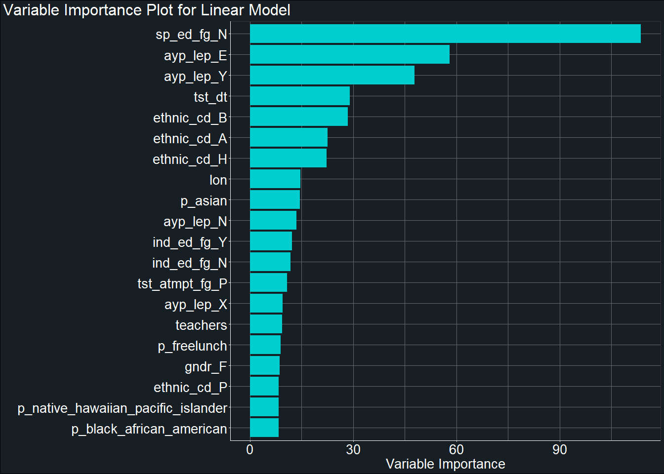
From the plot, we can see that the variable sp_ed_fg_N which indicates whether a student participates in an Individualized Education Plan was one of the most important predictor of students’ test score. Other important predictors include students’ Limited English Proficiency status and ethnicity.
Discussion
The linear model provided an introduction to machine learning and a general estimate of the RMSE model fit based on all of our predictor variables. Using the linear model, our predictors were able to account for 43.65% of the variance in our score with an RMSE of 86.98 in our left-out dataset.
Overall, the linear model was extremely quick to run computationally (only took 1.48 min to run through our 10-fold CV) as the algorithm makes a lot of assumptions about the data and there were no hyperparameter tuning involved in the linear model (we will briefly touch upon penalized regression which allows for tuning in the section below). Given that the linear model makes high assumption of the data, the linear model will have relatively low variance when applied to new unseen data. However, given the low-variance of the linear model, we will generally expect the model to produce consistent prediction that may not be the most accurate.
To improve our RMSE, we will explore application of non-linear models - Random Forest and Boosted Tree - to our data that can also be tuned for an optimal bias-variance balance.
Penalized Regression
As mentioned above, linear model makes high assumptions about the data and does not provide any hyperparameters for tuning bias-variance balance. Real world data may not necessarily fit with all the assumptions made by the linear model. One can look into penalized regression (also known as regularized regression or shrinkage method) to introduce bias or constraint in your model coefficients to reduce the variance and take into account a balanced bias.
Popular penalized regression methods include:
Ridge
Lasso
Elastic net
For more details on penalized regression, refer to Chapter 6, Regularized Regression of Hands-On Machine Learning with R by Boehmke & Greenwell (2020).